The CTX Device
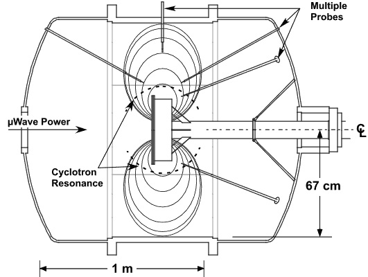
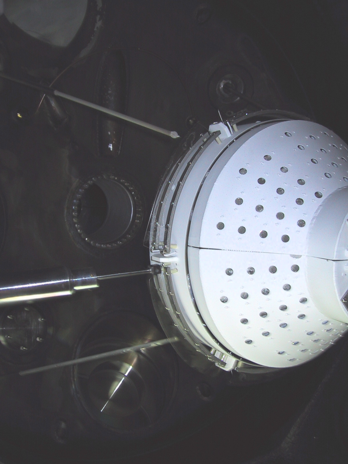
- Mechanically supported Dipole Magnet inside a vacuum chamber.
- Bmax ~15kG a the magnet face, and falls off (1/R3) to $\sim$50G at the chamber wall
- Electron Cyclotron Resonance Heating (ECRH) of 1kW @2.45GHz.
- A series of high impedence floating potential probes to measure global electrostatic mode structure.
- One moveable Langmuir Probe biased in the Ion Saturation Regime.
- Two moveable Mach probes to measure ion flow.
- The Polar Imager (PI) Array: An array of 96 Gridded Energy Analyzers, digitized at high speed, to measure the end-loss current to the dipole magnet.
- The Equitorial Mesh Biasing Array: 6 individual Tungsten meshes on the equitorial plane around the dipole magnet. The mesh array is used to drive radial current (E-field) which induces global E X B rotation in the azimuthal (Toroidal) direction. The meshes can be also be individually biased to create m=1 Non-axisymmetric Electric Field as well.
- A large moveable, spherical 'Bias Probe' to create a delta-function potential inside the vacuum chamber.
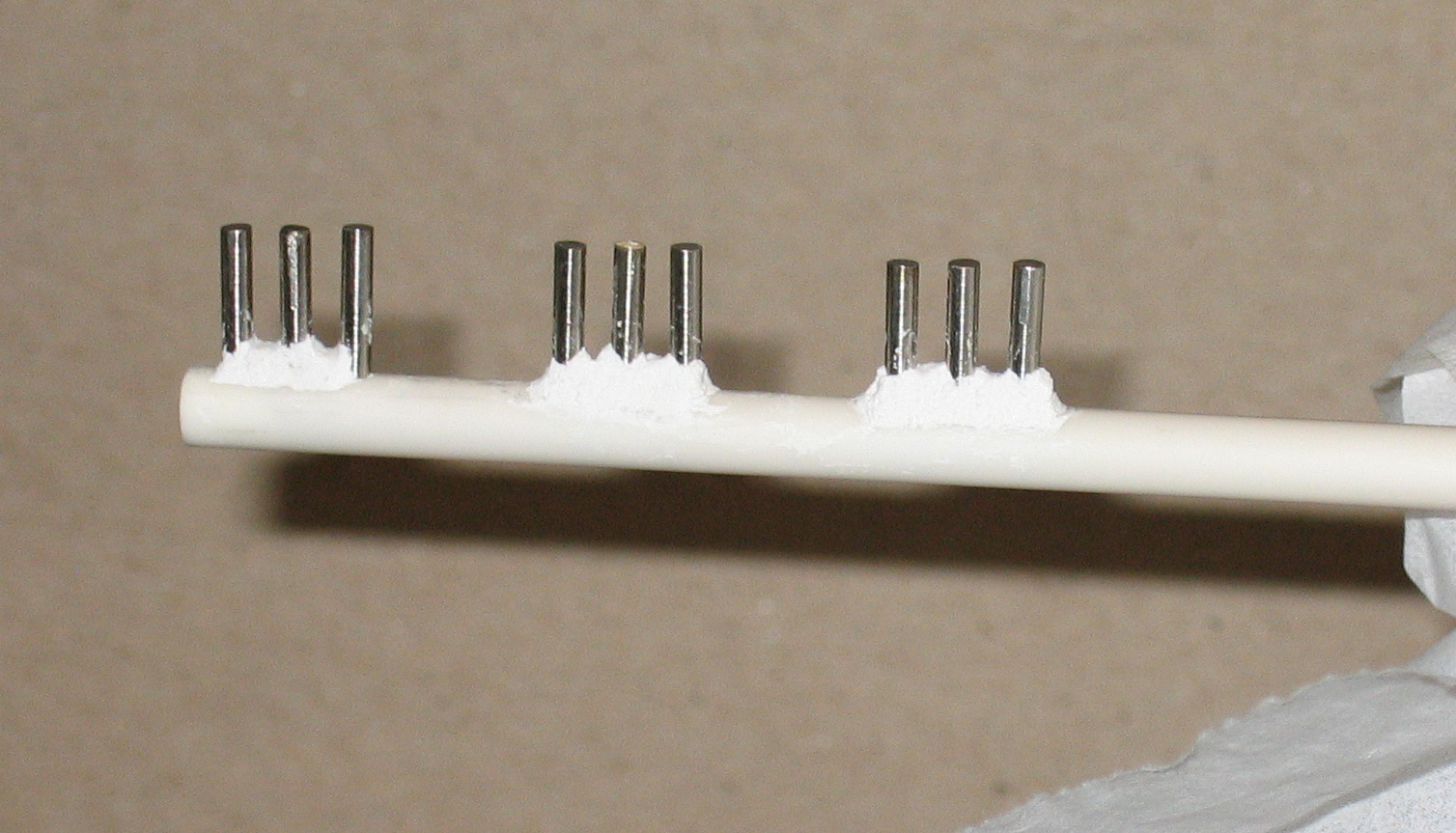
- One Triple Probe Array, consisting of three sets of three probe tips to simultanously measure floating potential, temperture, and density at three radial locations on the equitorial plane.
Basic Dipole Plasma Physics
Charged particle motion in a dipole separates into three motions.- Gyro (Cyclotron) Motion: Charged particles gyrate about magnetic field lines. This motion conserves the first adiabatic invariant $\mu=mv_\perp^2 / 2B$. Gyration has a characteristic frequency $\omega_c$
- Bounce Motion: The strength of the magnetic field in a dipole varies along a magnetic field line ( $\nabla_{||}B \neq 0$). Charged Particles 'bounce' along a field line between points of high magnetic field strength in a magnetic 'mirror'. This motion conserves the second adiabatic invariant $J=\int v_{||}ds$. Bounce motion has a characteristic frequency $\omega_b$.
-
 Drift Motion: The magnetic field has gradients perpendicular to B ($\nabla_\perp B \neq 0$), as well as magnetic curvature. Forces exist from magnetic gradients ($F=-\mu\nabla B$) and curvature (Centrifugal) which cause electrons and ions to drift in opposite directions. Drift motion has a characteristic frequency $\omega_d$
- The three motions separate: $\omega_d << \omega_b << \omega_c$
In a plasma confined by a dipole, a similar process occurs. Now it is not the force of grivity which drives the process, but the $\nabla B$ force, and the boundary is now the plasma-vacuum boundary which becomes distorted. Here, the feedback drive is the force which arises from the Electric field generated $E_1$ (due to counter drifting electrons and ions) crossed with the dipole magnetic field $B _0$. The Interchange Instability in a dipole is a 'Fluting Instability', causing perturbations with wave numbers predominantly in the azimuthal (toroidal) direction ($k _r, k_{||}=0, k_\varphi \neq 0$).
Hot Electron Interchange (HEI)
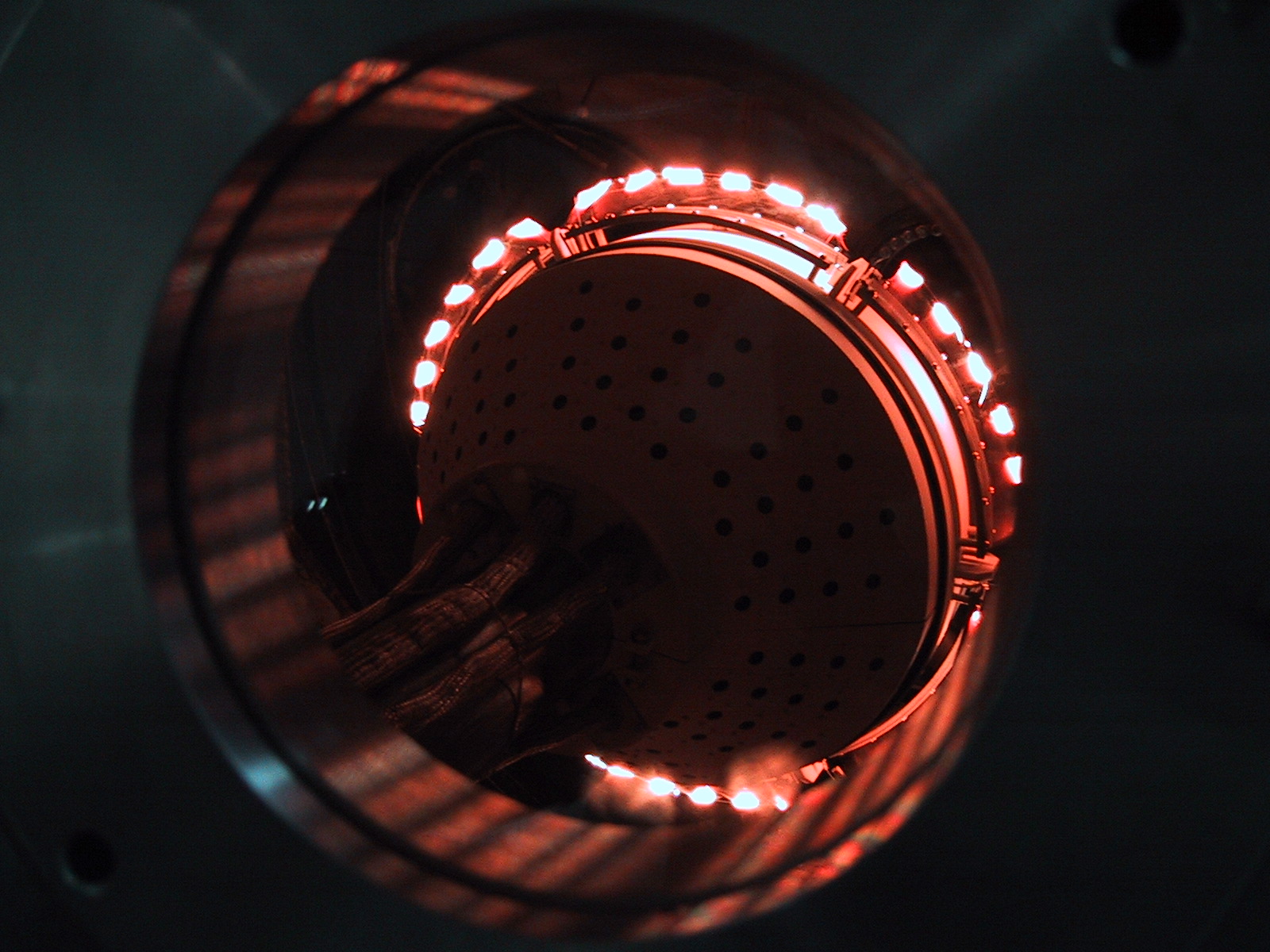
-In CTX, ECRH produces a hot population of energetic (10-40 keV), deeply trapped electrons. A so-called 'Artificial Radiation Belt', as seen in the Earth's Magnetosphere, as well as Jupiter.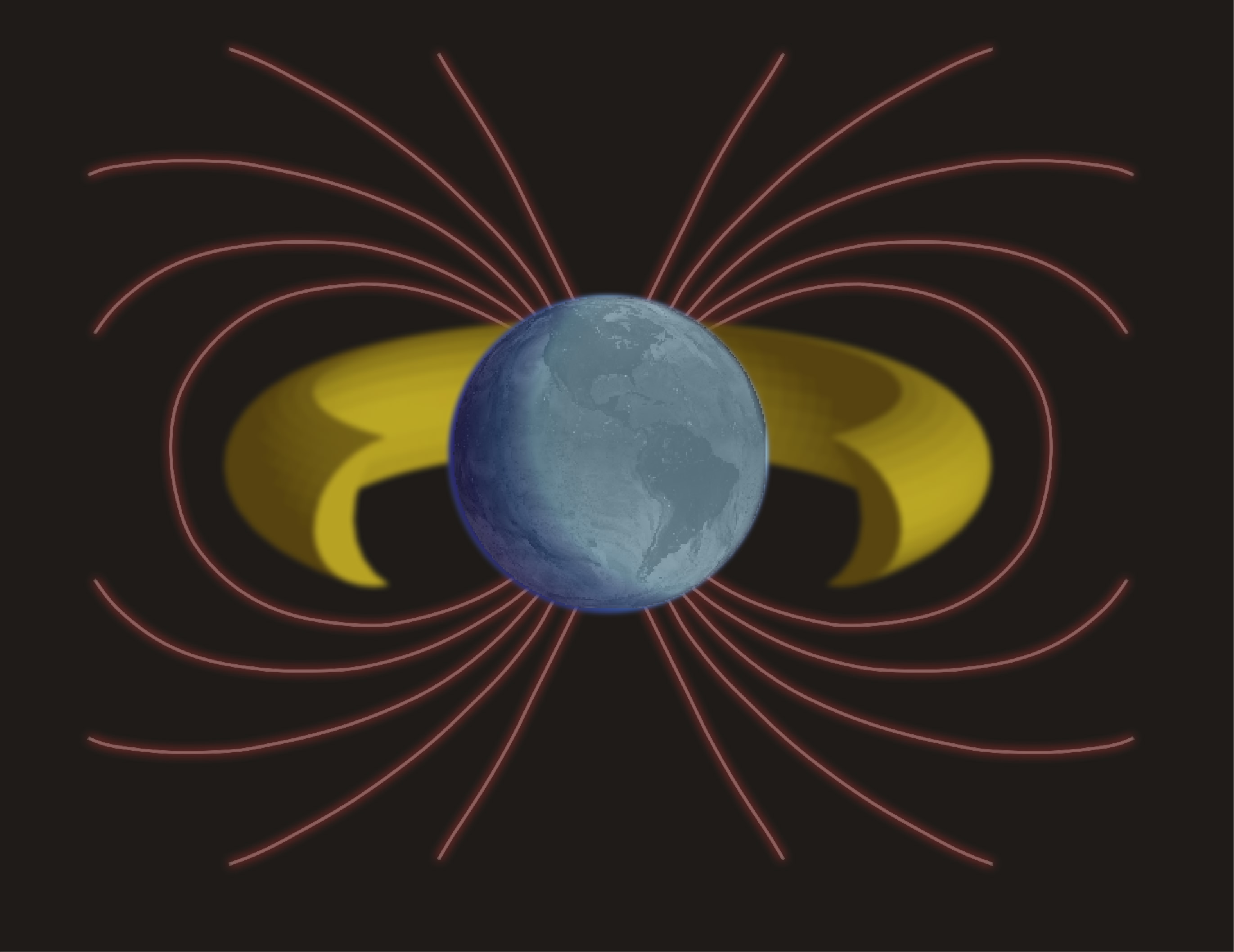
-The density of the hot electron population grows in time, until the density gradient is driven to an unstable value. Once the unstable limit is achieved, chaotic particle motion drives cross-field transport of hot electros (HEI burst). These bursts are detected by floating potential probes, and a large end-loss flux of electrons to the Polar Imager Array. After the chaotic burst, coherent, rotating modes are observed via floating potential measurements. These modes exhibit frequency sweeping, and a complex mode structure. A movie of such outward radial transport after the HEI burst can be seen here. Note the increased rotation frequency during the radial transport events.
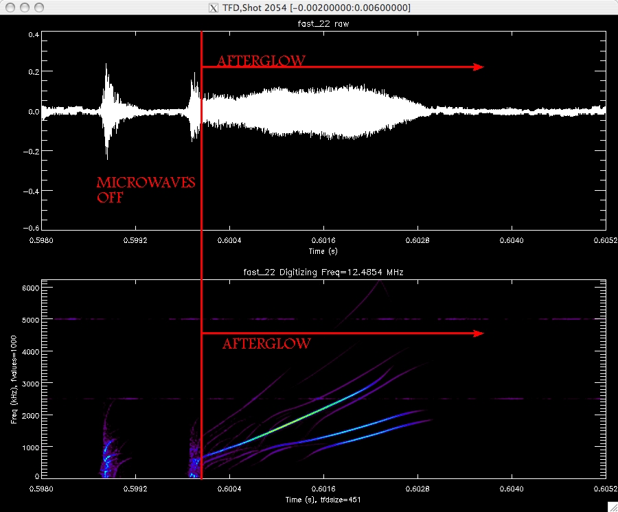
-During heating, the modal amplitude and frequency is limited, but in the 'Afterglow' after ECRH has been turned off, the mode is allowed to grow until the discharge is terminated.
Afterglow TFD 1
Sound file
Afterglow TFD 2
Sound File
Effects of Biasing
Movie of observed (electron gradB) drift resonant fluctuations.
-Frequency sweeping is observed. A constant rotation (30-40kHz) spontaneously begins to rise to a higher frequency, then relaxes to the original. This behavior is seen at the marginal Non-Axisymmetric Bias.
-These dynamics are correlated with the floating potential fluctuations.
 TFD of Temporal Eigenfunction from Bi-orthogonal Decomposition of PI signals displays frequency sweeping. The Decomposition is done for 70 gridded energy analyzers located at the pole of the Dipole Magnet.
 TFD of Flating potential over the same time period.
Density Regimes
When the CTX is sufficiently fueled, the plasma denisty transitions from the 'Low-Density' regime, to the 'High-Density' regime. This transition suppresses the HEI Instability and is marked by large 10-20kHz fluctuations in the electrostatic potential seen here by nine floating tips in a radial array, as well as a probe at a larger equatorial radius. A transition to this density regime can be seen in this movie.
Turbulence In CTX
The "high density" regime is characterized by intense fluctuations in density and potential which obey a power-law above a few kHz. This is typical of turbulence, or temporal chaos.The turbulence in CTX can be observed through the visible light emitted by the plasma. Because the fluctuations are much faster than a standard camera can view, we are using a high speed camera (Phantom v7.1) to view the plasma in slow motion.
A movie ("Download Link", and play in Quicktime) of the local plasma radius displays the raw image in false-color, as well as the fluctuation from the time-average.
A summary plot shows that the fluctuations are highest where the gradient is steepest, and where the heating zone is (ECRH).